Track Framework Tutorial
This section provides a comprehensive guide to using the Track (Semi-Lagrangian) Framework of ATMOS-BUD. The Track framework allows users to analyze the atmospheric budgets for systems that move significantly, such as cyclonic systems.
In this tutorial, we will use data from the Reg1 cyclone, which originated in southeastern Brazil and was documented in the article Dias Pinto, J. R., and R. P. da Rocha (2011), The energy cycle and structural evolution of cyclones over southeastern South America in three case studies, J. Geophys. Res., 116, D14112. The data for Reg1 comes from the NCEP reanalysis and covers the period from August 8 to August 14, 2005.
Preparing Your Environment
Before running the program, ensure that your environment is set up correctly. This includes activating the conda environment and preparing the input files.
1. Activate the Conda Environment:
Activate your conda environment to ensure all dependencies are available:
conda activate atmosbud
2. Prepare Input Files:
The track file and the namelist file must be correctly configured in the inputs/ directory. These files define the system’s trajectory and the settings for the NCEP reanalysis data.
- Track file:
The
trackfile specifies the position (latitude and longitude) of the cyclone for each time step. In this tutorial, we will use thetrack_Reg1-Representativefile for the Reg1 cyclone.
cp inputs/track_Reg1-Representative inputs/track
- Namelist file for NCEP-R2:
The
namelistfile contains the configuration for running the program with the NCEP reanalysis data. Ensure you use the correct namelist configuration for your data.
cp inputs/namelist_NCEP-R2 inputs/namelist
Once these steps are completed, you are ready to run the program with the Track (Semi-Lagrangian) Framework.
Running ATMOS-BUD with the Track Framework
To run ATMOS-BUD using the Track Framework, use the following command in your terminal:
python atmos_bud.py path-to-file/your_input_file.nc -t
Replace path-to-file/your_input_file.nc with the path to your NetCDF input file. For example, analyzing the Reg1 cyclone data:
python atmos_bud.py samples/Reg1-Representative_NCEP-R2.nc -t
Ensure that the namelist and track files are properly configured in the inputs/ directory. Results will be stored in the ATMOS-BUD_Results directory, and visualizations will be generated for further analysis.
Example Terminal Output
When you run the program, you will see detailed logs in the terminal. Below is an example output for the execution of the program, explaining the key components of the process:
2025-06-13 10:48:24,139 - atmos_bud - INFO - ⏳ Loading samples/Reg1-Representative_NCEP-R2.nc...
2025-06-13 10:48:24,477 - atmos_bud - INFO - ✅ Loaded samples/Reg1-Representative_NCEP-R2.nc successfully!
2025-06-13 10:48:24,478 - atmos_bud - INFO - 🔄 Preprocessing data...
2025-06-13 10:48:24,490 - atmos_bud - INFO - ✅ Preprocessing done.
2025-06-13 10:48:24,490 - atmos_bud - INFO - 🔄 Starting the computation of vorticity (zeta) and temperature tendencies...
2025-06-13 10:48:24,544 - atmos_bud - INFO - ✅ Computation completed successfully!
2025-06-13 10:48:24,544 - atmos_bud - INFO - Directory where results will be stored: ./Results/Reg1-Representative_NCEP-R2_track
2025-06-13 10:48:24,544 - atmos_bud - INFO - Directory where figures will be stored: ./Results/Reg1-Representative_NCEP-R2_track/Figures
2025-06-13 10:48:24,544 - atmos_bud - INFO - Name of the output file with results: Reg1-Representative_NCEP-R2_track
Explanation of Key Terminal Outputs
Loading and Preprocessing: The program first loads the input data (
samples/Reg1-Representative_NCEP-R2.nc), preprocesses it, and then begins the main computation (e.g., computing vorticity and temperature tendencies).
2025-06-13 10:43:51,977 - atmos_bud - INFO - ⏳ Loading samples/Reg1-Representative_NCEP-R2.nc...
2025-06-13 10:43:52,315 - atmos_bud - INFO - ✅ Loaded samples/Reg1-Representative_NCEP-R2.nc successfully!
2025-06-13 10:43:52,315 - atmos_bud - INFO - 🔄 Preprocessing data...
2025-06-13 10:43:52,327 - atmos_bud - INFO - ✅ Preprocessing done.
2025-06-13 10:43:52,327 - atmos_bud - INFO - 🔄 Starting the computation of vorticity (zeta) and temperature tendencies...
2025-06-13 10:43:52,382 - atmos_bud - INFO - ✅ Computation completed successfully!
- Time Step Processing:
For each time step, the program calculates atmospheric diagnostics, such as vorticity (ζ), geopotential height, and wind speed. It will also generate figures for each time step.
2025-06-13 10:43:52,394 - atmos_bud - INFO - ⏳ Processing time step: 2005-08-08 00Z
2025-06-13 10:43:52,644 - atmos_bud - INFO - 📍 central lat: -22.5, central lon: -45.0, size: 15.0 x 15.0, lon range: -52.5 to -37.5, lat range: -30.0 to -15.0
2025-06-13 10:43:52,644 - atmos_bud - INFO - 📍 850 hPa diagnostics --> min ζ: -1.71e-05, min geopotential height: 1563, max wind speed: 8.91
2025-06-13 10:43:52,644 - atmos_bud - INFO - 📍 850 hPa positions (lat/lon) --> min ζ: -17.50, -47.50, min geopotential height: -30.00, -42.50, max wind speed: -15.00, -37.50
- Generated Figures:
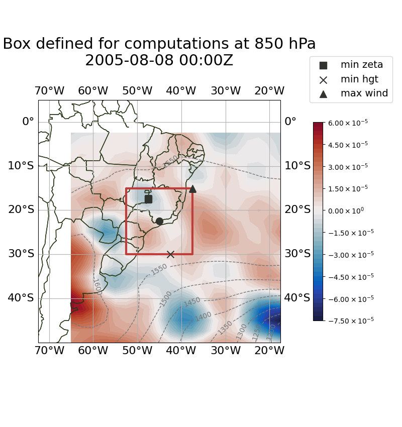
Figures will be created for each time step, showing the defined analysis box and relevant atmospheric diagnostics.
2025-06-13 10:43:53,531 - atmos_bud - INFO - 📊 Created figure with box defined for computations at box_200508080000.png
- Completion of Outputs:
After processing all time steps, the program will generate summary plots (e.g., time series, Hovmöller diagrams) and save all output files (CSV, NetCDF) in the appropriate directories.
2025-06-13 10:44:19,310 - atmos_bud - INFO - 📍 Created figure with track and boxes defined for computations: ./Results/Reg1-Representative_NCEP-R2_track/Figures/track_boxes.png
2025-06-13 10:44:19,527 - atmos_bud - INFO - 📈 Time series plot created and saved: ./Results/Reg1-Representative_NCEP-R2_track/Figures/timeseries_min_zeta_min_hgt_850hPa.png
2025-06-13 10:44:19,692 - atmos_bud - INFO - 🌍 Hovmöller diagram of mean zeta created and saved: ./Results/Reg1-Representative_NCEP-R2_track/Figures/hovmoller_mean_zeta.png
- Final Outputs:
Once the analysis is complete, the program will display a message showing the total time taken for the execution and list all the generated output files.
2025-06-13 10:44:19,762 - atmos_bud - INFO - 💾 ./Results/Reg1-Representative_NCEP-R2_track/Reg1-Representative_NCEP-R2_track.nc created successfully
2025-06-13 10:44:19,762 - atmos_bud - INFO - ⏱️ --- Total time for running the program: 28.305777072906494 seconds ---
By interpreting this output, users can confirm the successful loading of data, the processing of each time step, and the generation of output files for further analysis.
Understanding the Output Files
After running the program, several files and plots are generated. Below is an example of the output directory structure and some of the generated visualizations.
Figures Directory:
The
Figures/folder contains plots that visualize the defined analysis box and the atmospheric conditions within that box for each time step.
boxes/: This subfolder contains images of the defined domain box at different time steps. These images are similar to those in the Fixed Framework and show the region of interest for each time step.Example of a figure showing the defined box at 850 hPa for August 8, 2005:
track_boxes.png: This plot shows the track of the system, along with the boxes defined for computations.
hovmoller_mean_zeta.png: This is a Hovmöller diagram showing the mean vorticity (ζ) over time across the domain.
timeseries_min_zeta_min_hgt_850hPa.png: This plot contains the time series of the minimum vorticity (ζ) and minimum geopotential height (hgt) at 850 hPa (minimum or maximum values of vorticity and geopotential height, depending on the--track-vorticityand--track_geopotentialarguments). This figure is particularly useful for diagnosing the system’s behavior and detecting the phases of its life cycle.
NetCDF File:
ATMOS-BUD will generate a NetCDF file containing all the computed variables for the atmospheric budgets:
Reg1-Representative_NCEP-R2_track.nc: This file contains the results of the computations performed on the domain defined by thetrackfile.
Track File
track: This is the original track file used to define the cyclone’s path.Reg1-Representative_NCEP-R2_track_track.csv: This file is generated by the program and includes diagnostic variables for the system’s trajectory, computed for the selected pressure level (defined by the--levelargument) and based on the chosen diagnostics (minimum or maximum values of vorticity and geopotential height, depending on the--track-vorticityand--track_geopotentialarguments). The header of this file looks like:
time;Lat;Lon;length;width;min_zeta_850;min_hgt_850;max_wind_850
Where:
- time: Time step of the track.
- Lat: Latitude of the system’s center.
- Lon: Longitude of the system’s center.
- length and width: Dimensions of the box used for the analysis.
- min_zeta_850: Minimum vorticity at 850 hPa.
- min_hgt_850: Minimum geopotential height at 850 hPa.
- max_wind_850: Maximum wind speed at 850 hPa.
CSV Files:
In addition to the plots, ATMOS-BUD generates CSV files containing the diagnostic results. These files are organized in subdirectories by budget category: heat, moisture, and vorticity.
Each CSV file contains the following terms:
- Heat Budget (heat_terms/):
dTdt: Temperature tendency (K/s).Theta: Potential temperature (K).AdvHTemp: Horizontal advection of temperature (K/s).AdvVTemp: Vertical advection of temperature (K/s).Sigma: Static stability term (K/Pa).ResT: Residual of the thermodynamic equation (K/s).AdiabaticHeating: Estimated diabatic heating (W/kg).
- Vorticity Budget (vorticity_terms/):
Zeta: Relative vorticity (1/s).dZdt: Vorticity tendency (1/s).AdvHZeta: Horizontal advection of vorticity (1/s²).AdvVZeta: Vertical advection of vorticity (1/s²).Beta: Meridional gradient of the Coriolis parameter (1/m/s).vxBeta: Meridional advection of planetary vorticity (1/s²).DivH: Horizontal divergence of the wind (1/s).ZetaDivH: Term ζ·div(V) (1/s²).fDivH: Term f·div(V) (1/s²).Tilting: Tilting term (1/s²).ResZ: Residual of the vorticity budget (1/s²).
- Moisture Budget (moisture_terms/):
dQdt: Specific humidity tendency (kg/m²/s).dQdt_integrated: Vertically integrateddQdt(kg/m²/s).divQ: Horizontal divergence of moisture flux (1/s).divQ_integrated: Vertically integrateddiv(Q)(kg/m²/s).WaterBudgetResidual:dQdt_integrated+divQ_integrated(kg/m²/s).
Log File
The log file provides details about the execution process.
log.Reg1-Representative_NCEP-R2: Contains runtime information, including any errors or warnings encountered during execution.
By interpreting these outputs, users can analyze the cyclone’s life cycle and associated atmospheric budgets. The diagnostic plots and CSV files are valuable tools for understanding the behavior of the system over time.
Visualizing Generated Data
The process of visualizing the output data from the Track Framework is exactly the same as in the Fixed Framework. For detailed instructions on how to visualize the generated variables, please refer to the Visualizing Generated Data section in the Fixed Framework Tutorial.
- In summary:
Use the provided visualization scripts, such as
map_example.pyandvertical-profiles_example.py, to generate maps and vertical profile plots from the resulting NetCDF files and CSV data.These scripts can be found in the
plots/directory.